Data & Code/Visualisation/Country Ball Plot

Country Ball Plot

Overview

A scatter plot where each point is one country in one year, positioned by GDP per capita on the y-axis. The chart uses landmark years (every 5 years, 1980–2025) to keep the x-axis readable. The "fun" version renders the top-5 economies per year as circular country flag images — the "country ball" effect — using matplotlib, PIL, and a GitHub-hosted flag CDN. The clean version uses ISO3 text labels instead, with no external image dependency.

Data is pulled live from the IMF World Economic Outlook via sdmx using indicator NGDPDPC (GDP per capita, current USD) for all 54 ECA member countries. No CSV, no local data dependency. The API is queried by country key rather than all — faster and avoids pulling the entire world dataset.

Variant	Extra dependencies	Internet at plot time	Best for
Flag markers	`pillow` `requests`	Yes — fetches flags at render	Presentations, reports
ISO3 labels	None beyond core stack	No	Publications, offline use

Flag markers

Needs internet

The top-5 GDP per capita economies per year are rendered as flag images fetched from CSS-Country-Flags-Rounded by matahombres using OffsetImage and AnnotationBbox. Remaining countries appear as small grey dots. If a flag fetch fails, the script falls back gracefully to a labelled dot.

Internet required at render time. Each unique flag is fetched once and cached in the session. Running offline will trigger the dot fallback for all markers.

African GDP per capita country ball plot — clean version — Sample output — 31 Mar 2026. Top 5 per year labelled in steelblue.

Download Jupyter notebook · country_ball_plot.ipynb

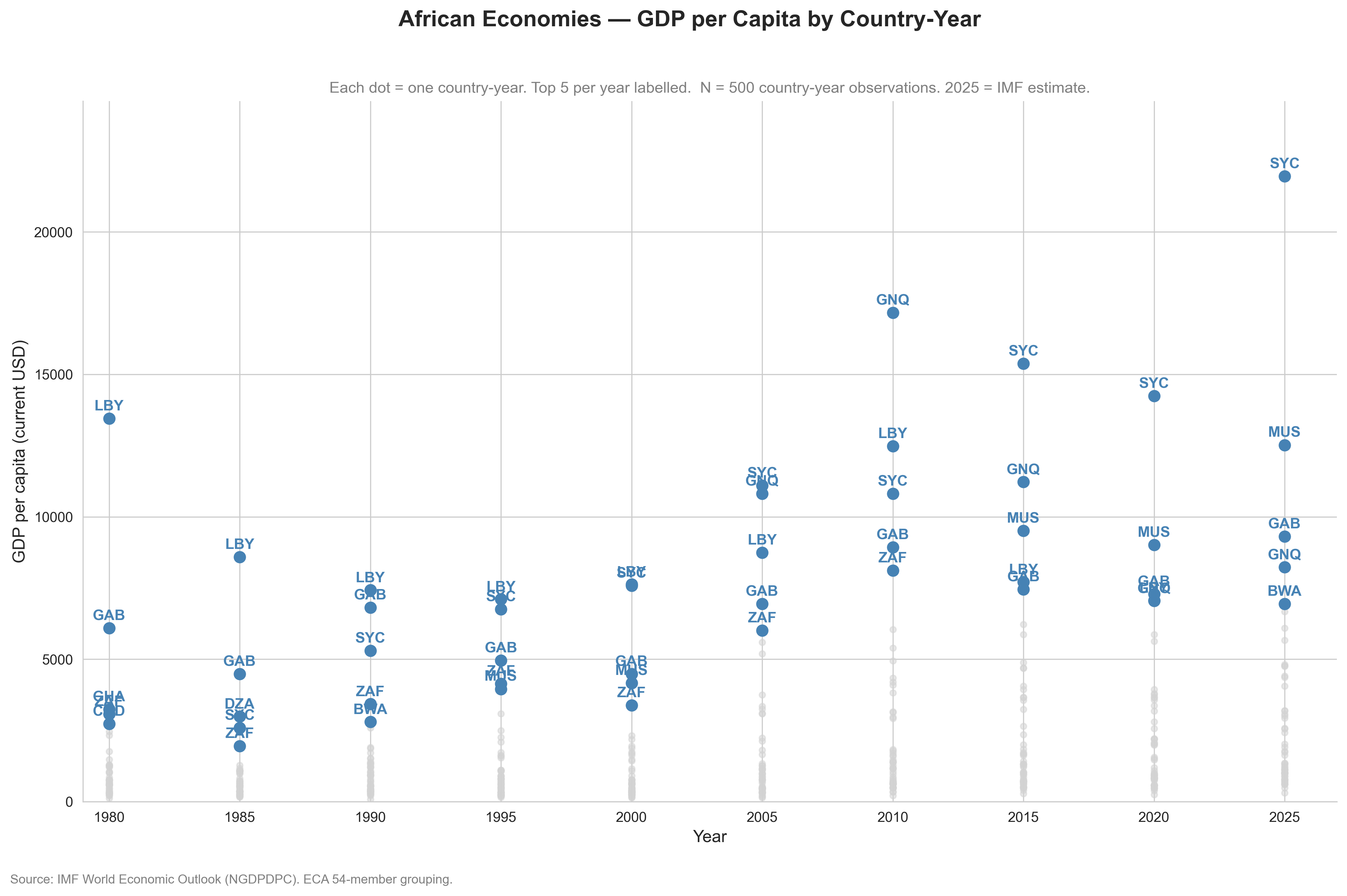
Python · GDP per capita — flag version

IMF WEO → ECA54 → landmark years → flag markers for top 5.

Python

1# pip install sdmx1 pillow requests pycountry seaborn
2import sdmx
3import pandas as pd
4import numpy as np
5import matplotlib.pyplot as plt
6import seaborn as sns
7import pycountry
8import requests
9from PIL import Image
10from io import BytesIO
11from matplotlib.offsetbox import OffsetImage, AnnotationBbox
12from datetime import datetime
13
14# ── 1. Country list ───────────────────────────────────────────────────────
15ECA54_ISO3 = [
16    "DZA","AGO","BEN","BWA","BFA","BDI","CPV","CMR","CAF","TCD","COM",
17    "COG","COD","CIV","DJI","EGY","ERI","ETH","GNQ","GAB","GMB","GHA",
18    "GIN","GNB","KEN","LSO","LBR","LBY","MDG","MWI","MLI","MRT","MUS",
19    "MAR","MOZ","NAM","NER","NGA","RWA","STP","SEN","SYC","SLE","SOM",
20    "ZAF","SSD","SDN","TZA","TGO","TUN","UGA","ZMB","ZWE","SWZ"
21]
22
23# Landmark years only — keeps the plot uncluttered
24target_years = {1980, 1985, 1990, 1995, 2000, 2005, 2010, 2015, 2020, 2025}
25
26# ── 2. Fetch IMF WEO ─────────────────────────────────────────────────────
27# NGDPDPC = GDP per capita, current USD.
28# Country-key query (ECA54.NGDPDPC.A) is faster than key="all".
29IMF_DATA = sdmx.Client("IMF_DATA")
30ECA54    = "+".join(ECA54_ISO3)
31
32resp = IMF_DATA.data(
33    "WEO",
34    key   = f"{ECA54}.NGDPDPC.A",
35    params= {"startPeriod": 1980, "endPeriod": 2025},
36)
37
38ser = sdmx.to_pandas(resp)
39df  = ser.rename("value").reset_index() if isinstance(ser, pd.Series) else ser.copy()
40df  = df.rename(columns={"COUNTRY": "ISO3", "TIME_PERIOD": "year"})
41
42keep = [c for c in ["ISO3", "year", "value"] if c in df.columns]
43df   = df[keep]
44
45df["year"]  = pd.to_datetime(df["year"].astype(str), errors="coerce").dt.year
46df["value"] = pd.to_numeric(df["value"], errors="coerce")
47df["year"]  = pd.to_numeric(df["year"],  errors="coerce").astype("Int64")
48df = df[df["year"].isin(target_years)].copy()
49df = df.dropna(subset=["value"])
50
51# ── 3. ISO2 + rank ────────────────────────────────────────────────────────
52df["ISO2"] = df["ISO3"].apply(
53    lambda x: pycountry.countries.get(alpha_3=x).alpha_2
54    if pycountry.countries.get(alpha_3=x) else None
55)
56# Namibia edge case: pycountry returns None for "NA" (looks like null)
57df.loc[df["ISO3"] == "NAM", "ISO2"] = "NA"
58
59df["rank"] = df.groupby("year")["value"].rank(method="first", ascending=False)
60top5   = df[df["rank"] <= 5].copy()
61others = df[df["rank"] >  5].copy()
62
63mask = (df["rank"] <= 5) & (df["ISO2"].isna())
64print(f"{mask.sum()} missing ISO2 in top-5" if mask.any() else "Safe to proceed")
65
66# ── 4. Flag helper ────────────────────────────────────────────────────────
67# Cache PIL Image, not OffsetImage — OffsetImage artists cannot be reused
68# across ax.add_artist() calls; doing so silently moves rather than copies.
69# Flags: github.com/matahombres/CSS-Country-Flags-Rounded
70flag_cache: dict = {}
71
72def get_flag_image(iso2: str, zoom: float = 0.045):
73    if pd.isna(iso2):
74        return None
75    iso2 = str(iso2).upper()
76    if iso2 not in flag_cache:
77        try:
78            url  = (f"https://raw.githubusercontent.com/matahombres/"
79                    f"CSS-Country-Flags-Rounded/master/flags/{iso2}.png")
80            r    = requests.get(url, timeout=5)
81            flag_cache[iso2] = (
82                Image.open(BytesIO(r.content)).convert("RGBA")
83                if r.status_code == 200 else None
84            )
85        except Exception:
86            flag_cache[iso2] = None
87    img = flag_cache[iso2]
88    return OffsetImage(img, zoom=zoom) if img is not None else None
89
90# Pre-fetch all unique flags before plotting
91for iso2 in top5["ISO2"].dropna().astype(str).str.upper().unique():
92    get_flag_image(iso2)
93
94# ── 5. Plot ───────────────────────────────────────────────────────────────
95sns.set_style("whitegrid")
96fig, ax = plt.subplots(figsize=(16, 9))
97
98# Non-top-5: single vectorised call (fast)
99ax.scatter(
100    others["year"], others["value"],
101    s=18, color="lightgrey", alpha=0.6, zorder=2
102)
103
104# Top-5: flag markers, fallback to labelled dot
105for row in top5.itertuples(index=False):
106    x, y = row.year, row.value
107    flag = get_flag_image(row.ISO2)
108    if flag:
109        ax.add_artist(AnnotationBbox(flag, (x, y), frameon=False))
110    else:
111        ax.scatter(x, y, s=60, color="steelblue", zorder=3)
112        ax.text(x, y + 30, row.ISO3, fontsize=7, ha="center", color="steelblue")
113
114# ── 6. Labels & formatting ────────────────────────────────────────────────
115ax.set_xlabel("Year", fontsize=12)
116ax.set_ylabel("GDP per capita (current USD)", fontsize=12)
117y_max = df["value"].max()
118ax.set_ylim(0, y_max * 1.12)
119ax.set_xlim(min(target_years) - 1, max(target_years) + 2)
120ax.set_xticks(sorted(target_years))
121fig.suptitle(
122    "African Economies — GDP per Capita by Country-Year",
123    fontsize=16, fontweight="bold"
124)
125ax.set_title(
126    f"Each marker = one country-year. Top 5 per year shown as flag.  "
127    f"N = {len(df)} country-year observations. 2025 = IMF estimate.",
128    fontsize=11, color="grey"
129)
130fig.text(
131    0.08, 0.02,
132    "Source: IMF World Economic Outlook (NGDPDPC). ECA 54-member grouping.",
133    fontsize=9, color="grey", ha="left"
134)
135sns.despine()
136
137today = datetime.today().strftime("%d%b%Y")
138plt.savefig(f"Africa_GDPpc_countryball_{today}.png", dpi=300, bbox_inches="tight")
139plt.show()

ISO3 labels

No internet required

Same data pipeline and ranking logic, but the top-5 countries per year are drawn as coloured dots with ISO3 text labels. Colours are assigned persistently — a country that appears in the top 5 across multiple landmark years always gets the same colour, making it easy to track economies over time.

Download Jupyter notebook · country_ball_plot.ipynb

Python · GDP per capita — clean version

IMF WEO → ECA54 → landmark years → ISO3 labels for top 5.

Python

1# pip install sdmx1 pycountry seaborn
2# Same data pipeline as the flag version — no pillow or requests needed.
3import sdmx
4import pandas as pd
5import numpy as np
6import matplotlib.pyplot as plt
7import seaborn as sns
8import pycountry
9from datetime import datetime
10
11# ── 1. Country list & target years ───────────────────────────────────────
12ECA54_ISO3 = [
13    "DZA","AGO","BEN","BWA","BFA","BDI","CPV","CMR","CAF","TCD","COM",
14    "COG","COD","CIV","DJI","EGY","ERI","ETH","GNQ","GAB","GMB","GHA",
15    "GIN","GNB","KEN","LSO","LBR","LBY","MDG","MWI","MLI","MRT","MUS",
16    "MAR","MOZ","NAM","NER","NGA","RWA","STP","SEN","SYC","SLE","SOM",
17    "ZAF","SSD","SDN","TZA","TGO","TUN","UGA","ZMB","ZWE","SWZ"
18]
19target_years = {1980, 1985, 1990, 1995, 2000, 2005, 2010, 2015, 2020, 2025}
20
21# ── 2. Fetch IMF WEO ─────────────────────────────────────────────────────
22IMF_DATA = sdmx.Client("IMF_DATA")
23ECA54    = "+".join(ECA54_ISO3)
24
25resp = IMF_DATA.data(
26    "WEO",
27    key   = f"{ECA54}.NGDPDPC.A",
28    params= {"startPeriod": 1980, "endPeriod": 2025},
29)
30
31ser = sdmx.to_pandas(resp)
32df  = ser.rename("value").reset_index() if isinstance(ser, pd.Series) else ser.copy()
33df  = df.rename(columns={"COUNTRY": "ISO3", "TIME_PERIOD": "year"})
34
35keep = [c for c in ["ISO3", "year", "value"] if c in df.columns]
36df   = df[keep]
37
38df["year"]  = pd.to_datetime(df["year"].astype(str), errors="coerce").dt.year
39df["value"] = pd.to_numeric(df["value"], errors="coerce")
40df["year"]  = pd.to_numeric(df["year"],  errors="coerce").astype("Int64")
41df = df[df["year"].isin(target_years)].copy()
42df = df.dropna(subset=["value"])
43
44# ── 3. Rank & assign persistent colours ──────────────────────────────────
45df["rank"] = df.groupby("year")["value"].rank(method="first", ascending=False)
46
47# Countries appearing in top-5 at any point get a fixed colour across years
48top_countries = df[df["rank"] <= 5]["ISO3"].unique()
49palette       = sns.color_palette("husl", len(top_countries))
50color_map     = dict(zip(top_countries, palette))
51
52top5   = df[df["rank"] <= 5].copy()
53others = df[df["rank"] >  5].copy()
54
55# ── 4. Plot ───────────────────────────────────────────────────────────────
56sns.set_style("whitegrid")
57palette       = sns.color_palette("husl", len(top_countries))
58color_map     = dict(zip(top_countries, palette))
59
60fig, ax = plt.subplots(figsize=(16, 9))
61
62ax.scatter(
63    others["year"], others["value"],
64    s=18, color="lightgrey", alpha=0.5, zorder=2
65)
66
67for row in top5.itertuples(index=False):
68    x, y = row.year, row.value
69    ax.scatter(x, y, s=60, color="steelblue", zorder=3)
70    ax.text(x, y + 280, row.ISO3, fontsize=10.5,
71            ha="center", color="steelblue", fontweight="bold")
72
73# ── 5. Labels & formatting ────────────────────────────────────────────────
74ax.set_xlabel("Year", fontsize=12)
75ax.set_ylabel("GDP per capita (current USD)", fontsize=12)
76y_max = df["value"].max()
77ax.set_ylim(0, y_max * 1.12)
78ax.set_xlim(min(target_years) - 1, max(target_years) + 2)
79ax.set_xticks(sorted(target_years))
80fig.suptitle(
81    "African Economies — GDP per Capita by Country-Year",
82    fontsize=16, fontweight="bold"
83)
84ax.set_title(
85    f"Each dot = one country-year. Top 5 per year labelled.  "
86    f"N = {len(df)} country-year observations. 2025 = IMF estimate.",
87    fontsize=11, color="grey"
88)
89fig.text(
90    0.08, 0.02,
91    "Source: IMF World Economic Outlook (NGDPDPC). ECA 54-member grouping.",
92    fontsize=9, color="grey", ha="left"
93)
94sns.despine()
95
96today = datetime.today().strftime("%d%b%Y")
97plt.savefig(f"Africa_GDPpc_countryball_clean_{today}.png", dpi=300, bbox_inches="tight")
98plt.show()

Notes & gotchas

Namibia ISO2 edge case

pycountry returns None for Namibia because its ISO2 code "NA" is interpreted as a null value in some contexts. Both scripts hardcode the fix: df.loc[df["ISO3"] == "NAM", "ISO2"] = "NA". Watch for the same issue with any ISO2 code that looks like a reserved word if you extend to other country lists.

Cache PIL Image, not OffsetImage

OffsetImage artists cannot be reused across multiple ax.add_artist() calls — doing so silently moves the artist rather than copying it. The fix is to cache the raw PIL.Image and instantiate a fresh OffsetImage each time. A country appearing across 10 landmark years still makes only one HTTP request.

Y-axis ceiling

The scripts set ax.set_ylim(0, y_max * 1.12) dynamically. Without this, a hardcoded ceiling will clip high-income outliers like Seychelles or Equatorial Guinea off the top of the plot — they appeared visually absent even though the data was present.

IMF WEO coverage gaps

Not all 54 African countries report to WEO every year. South Sudan (SSD), Eritrea (ERI), and Somalia (SOM) have sparse series and may not appear in early landmark years. Check df["ISO3"].value_counts() after the fetch to confirm coverage.

2025 value is an IMF estimate

The WEO includes projections for the current year. The 2025 data point is an IMF forecast, not outturn data — this is noted in the chart subtitle. Remove 2025 from target_years if you want observed data only.

Tuning the flag zoom

The zoom=0.045 parameter controls flag size relative to the axes. At 16:9 / 300 dpi this gives roughly a 40px flag. Increase to 0.07 for presentation slides; reduce to 0.025 for dense multi-panel figures.